Disclaimer: this post was written before I learned that pie charts are bad.
As some of you might recall, I have been talking about visualizing digital music collections using Microsoft tools. It all started back in the days of Pivot Viewer (At some point I was even part of a lustrous duo called ‘the Pivot Brothers’).
Now, with Power BI being just around the corner I started thinking about taking on this old habit again. Here it goes…
If you are like me you have a digital music collection all nice and tidy complete with ID3 tags. A lot of tools exist that enable you to work with these tags and fix them. I particularly like Mp3tag (http://www.mp3tag.de/en/) which is free and is extensible. It also comes with an export function to CSV, although it does not export enough to my taste. I created my own export file and I suggest you do too. Keep reading if you want to know how and maybe rip mine.
Of course you can use any other tool that has an export function, as long as you end up with something like a CSV. If you want to follow along in my step-by-step scenario I suggest installing Mp3tag.
Creating the export
Again, please note that you do not have to follow these steps exactly. If you use another tool (not Mp3tag) or already have an export file you would like to use skip to the next step.
To create the export with Mp3tag, open the program and navigate to where you music is stored (my collection sits on \192.168.1.9\Music, which is a folder on my server). Once Mp3tag has listed all your files (might take a while if you have a large collection), select all files (EditàSelect all files or CTRL+A) and then choose File à Export (CTRL+E). You will get the Export dialog. Now, hit the first button on the right (the little page with a star to create a new export configuration and give it a name (I named mine “My CSV Export”) and click OK. Notepad will open and allow you to edit the export configuration.
At this point you can copy and paste the code below into Notepad and hit save.
Then, return to Mp3tag, select your export configuration, set up the export file name and click OK. Wait for a while and then click No to not display the export file.
Loading the file
If you followed along you will have a CSV file that contains the export of your music collection delimited by semicolons. Your delimiter may be different. As a consequence the steps you need to take to get the data loaded may vary.
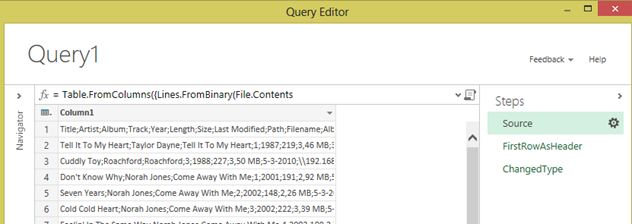
Open up Excel 2013, click on Power Query in the ribbon and select From File à From CSV. Select the CSV file you just created and click OK. Now Power Query will do its best to give you what you want but as you can see it is not very successful (with the build available at the time of this writing).
All is not lost however, because now we get to work with the magic of Power Query!
First off, we need to get rid of all the errors we get in the data rows. Click open the steps fly-out on the right and click the first step (Source) and click the icon right next to it. Then in the ‘Open file as’ drop down box select ‘Text File’ instead of ‘CSV Document’ and click OK. This already looks a lot better, doesn’t it?
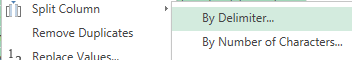
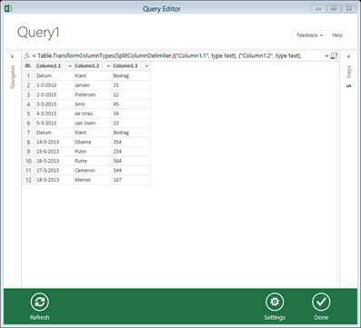
Now we need to split the column in by the semicolon delimiter. Make sure the ‘Source’ step is still selected and then right click on the ‘Column1’ header and choose ‘Split Column’ à ‘By Delimiter…’
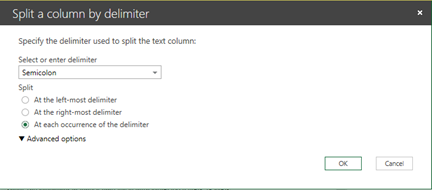
Make sure to select the correct delimiter (semicolon in my case) and make sure that ‘At each occurrence of the delimiter’ under ‘Split’ and click OK.
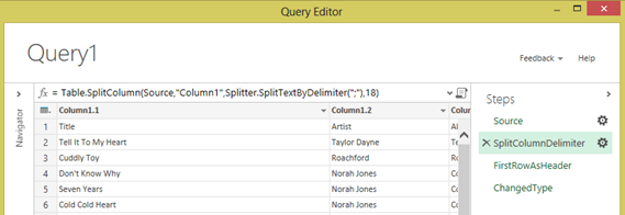
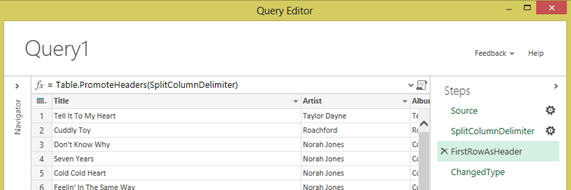
Then you screen should look like this:
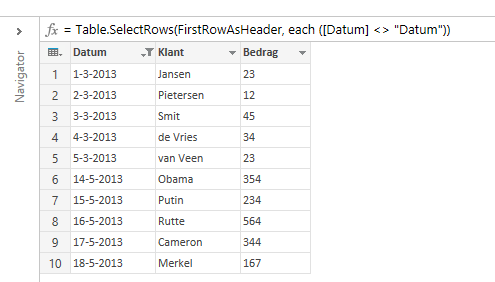
Now select the ‘FirstRowAsHeader’ step and check the output.
We now need to delete the last step (we will redo it ourselves later on). To do this mouse over and click on the little cross icon in front ‘ChangedType’.
Transforming the data
Change data types
Now we need to change some data types but right clicking on the header of the column and choosing ‘Change Type’ and choosing the type you want to change to.
Change these columns to the indicated types:
Column
Change to type
Last Modified
Date
BPM
Number (select 'Using locale' first and then select 'Number' and 'English (United States)' if your country does not use a . as decimal separator.
Bitrate
Number
Year
Number
Fix the Size column
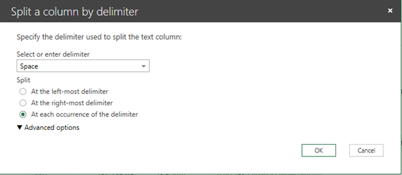
Now, split the Size column by right clicking on the ‘Size’ column header and selecting ‘Split Column’ and then ‘By Delimiter…’. Select ‘Space’ as delimiter and select ‘At the left-most delimiter’ as split option and click OK.
You will now get two size columns: Size.1 which contains the numerical value and Size.2 which contains MB or KB.
First, change Size.1 to a number (right click on header, Change Type à Number). Then insert a new column (right click on a column header, Insert Column à Custom…) and enter the following custom column formula:
if [Size.2] = "MB" then [Size.1]*1024 else [Size.1]
Rename the Custom column by right-clicking the header and choosing ‘Rename…’. Enter ‘Size’ as your column name and hit enter. You now have got a single column that reports the size of the song in Kb.
To wrap things up right click ‘Size.1’ and click ‘Remove’. Do the same for ‘Size.2’.
Add cover art
One of the nicest things of albums is the cover art. Luckily Windows stores the cover art in the same directory as your music files as a hidden file named ‘Folder.jpg. Let’s add this by adding another column (right click on a column header, choose Insert Column à Custom…) and entering the following custom formula:
[Path]& "Folder.jpg"
Rename the column to Cover.
Now we’re done transforming the data. The steps you performed form a script, which you can see by clicking on the title scroll icon at the formula bar. Here is my script:
As you can see every little step we took is represented in the script.
Now click ‘Done’ to get the transformed data in Excel, where we will start on the visualization.
Fixing the covers using PowerPivot and adding release date
Now we need to tell Power BI to read the cover column as a reference to an image. This is something we cannot do in Power Query at the moment, but we can in PowerPivot. In Excel, click PowerPivot à Manage to open up the PowerPivot window. In here, select your Cover column, go to Advanced and set the Data Category to be Image URL.
Also, add a new column (by clicking on the empty column at the right of your table) and enter the following formula:
=DATE([Year];1;1)
Hit enter and name this column ReleaseDate.
Building the visualization
Back in Excel, click Insert à Power View and start building your visualizations. Here are some examples I built:
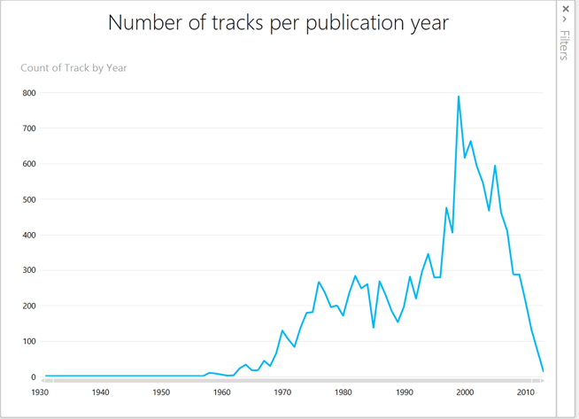
Number of tracks per release year
Count of track by year in a line graph
Apparently most the tracks in my collection were released around 2000, while the oldest track I have has been released in 1930.
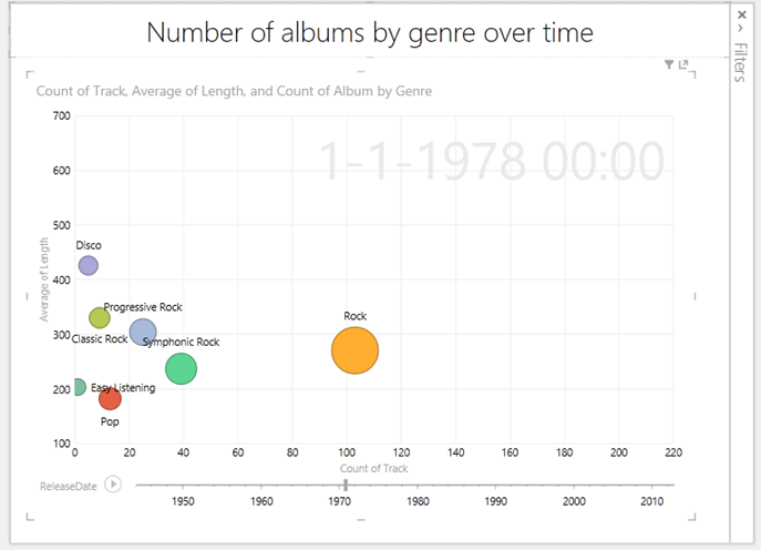
Number of tracks per genre over time
This clearly shows that in 1978 the rock genre was most popular (at least in the albums in my collection). However, the Disco songs were the longest on average.
The play axis at the bottom allows me to play through my collection over time.
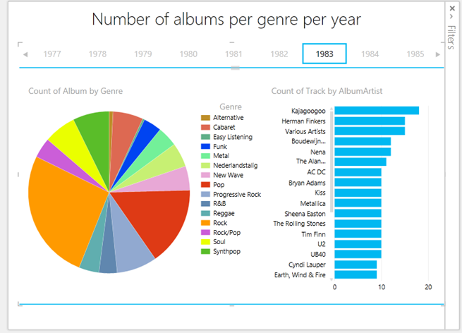
Number of albums per genre per year
In 1983 the most popular artist was Kajagoogoo and you also get an idea of what the popular genre was. (Yes, I am using a pie chart here, this was years ago.)
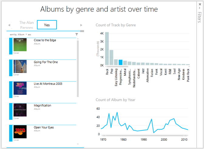
Albums by genre and artist of time
This shows the progressive rock genre and when it was popular. Also it shows which artists released albums categorized as progressive rock and which albums I have of that artist (I selected Yes).
That’s it
I will revisit visualizing my music collection when I have access to a BI Site, so I can show the latest visualization live. For now, this it it. Enjoy!
If you installed SQL 2012 you have probably noticed that you development environment for Integration Services, Analysis Services and Reporting Services is still hosted in a Visual Studio 2010 shell (SQL Server Data Tools). However, with a free download you can get the Microsoft Business Intelligence Project Templates for SSIS, SSAS and SSRS in your Visual Studio 2012 installation. All you need to do is to download and install it.
Being able to do this is very handy if you have multiple Excel sheets reporting on different periods, regions or products and you want to combine the data from those sheets into one table to use in your reporting.
First we need to make sure that ‘Advanced Query Editing’ is enabled. To do this, open Excel, go to the Power Query tab and choose Options. Then make sure the checkmark for ‘Advanced Query Editing’ is enabled. In order to successfully combine multiple Excel sheets we will need to modify the query’s script.
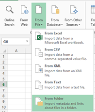
Just like with combining text files using Power Query, get started by clicking ‘From File’ and then ‘From Folder’.
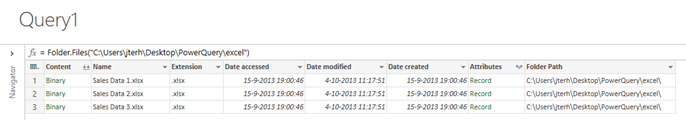
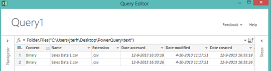
Specify the folder where your Excel files are located and choose ‘OK’.
As before Power Query returns the list of Excel files in the folder:
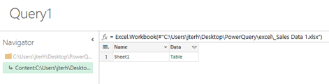
Lets click on the first cell of the first row to get the sheets of the Excel workbook:
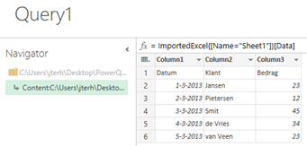
If you now click on ‘Table’ in ‘Data’ column of the Sheet1 row you will get the contents of the sheet itself:
Let’s first fix the headers. Right-click on the little table icon in the top left and choose ‘Use First Row As Headers’.
Now, in order to load the rest of the Excel files we need to modify the code a bit. To do this click on the little script icon just above the table:
The query editor opens and shows the M-script you have generated in the previous steps. Here is mine:
let
Source = Folder.Files("C:\Users\jterh\Desktop\PowerQuery\excel"),
#"C:\Users\jterh\Desktop\PowerQuery\excel\_Sales Data 1.xlsx" = Source{[#"Folder Path"="C:\Users\jterh\Desktop\PowerQuery\excel\",Name="Sales Data 1.xlsx"]}[Content],
ImportedExcel = Excel.Workbook(#"C:\Users\jterh\Desktop\PowerQuery\excel\_Sales Data 1.xlsx"),
Sheet1 = ImportedExcel{[Name="Sheet1"]}[Data],
FirstRowAsHeader = Table.PromoteHeaders(Sheet1)
in
FirstRowAsHeader
If we take a closer look at this M-script we see the following structure:
let
 A = f(x),
 B = f(A),
 C = f(B)
 in C
What happens is that we define A and then in steps apply functions on A. In each step we take as input the output of the previous step. In the end we return the result of the last function.
The M-script above is quite static in the sense that it applies only to the Excel sheet we selected (in this case ‘Sales Data 1.xlsx’). What we need to do is find a way to provide a parameter to this code and execute the code for every Excel sheet in the directory.
To make this work we will need to define a function based on the M-script we currently have. To do that we need to change the M-script to:
let ExcelFile = (FilePath, FileName) =>
let
    Source = Folder.Files(FilePath),
    File = Source{[#"Folder Path"=FilePath,Name=FileName]}[Content],
    ImportedExcel = Excel.Workbook(File),
    Sheet1 = ImportedExcel{[Name="Sheet1"]}[Data],
    FirstRowAsHeader = Table.PromoteHeaders(Sheet1)
in
    FirstRowAsHeader
in
    ExcelFile
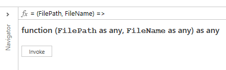
What we do here is defining a function with two parameters (the path to the files and a filename). Make sure you match the casing of ‘in’ and ‘let’ correctly! Do not use any capitals. Change your M-script accordingly and click ‘Done’.
Your Query Editor should now look like this:
Now, let’s make sure we understand what this query does by changing the name from ‘Query1’ to something like ‘GetExcel’ by double clicking on ‘Query1’ in this screen and entering the new name. We will use this name to invoke the function.
Click ‘Done’. We will invoke this function in a just a little while.
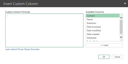
On the Power Query tab click ‘From File’ and choose ‘From Folder’ again. Re-enter the folder where your Excel files are stored and click ‘OK’. Now right-click a colum header and choose ‘Insert Column’ and choose ‘Custom…’. A formula editing screen opens:
Here we will need to invoke the function we defined earlier by entering the following:
GetExcel([Folder Path],[Name])
Click ‘OK’ and rename the column by right-clicking the column name and choosing ‘Rename’. I renamed the column to ‘FileContents’:
Now click the icon to select the columns to expand from your Excel sheet and click ‘OK’.
Now we have the contents of the files combined with information about the files in one table. To get rid of all columns except for the contents select the three contents columns, right-click and select ‘Remove Other Columns’:
Optionally you can rename the columns. When done click ‘Done’ to get the data in Excel.
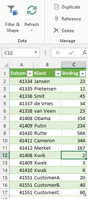
The best part is that if you add a sheet to the directory and click ‘Refresh’ in the Query tab of the ribbon, the data will get added to the result set:
So, if you have set this up and new data needs to be added as long as the structure of your Excel sheets does not change you can just click ‘Refresh’ and it works! This is the amazing power of Power Query.
For the information in this post I am heavily indebted to Michiel Rozema who originally figured this out.
In this post we will have a look at how text (CSV) files in a folder can be combined using Power Query for Excel. In a later post will we extend this and load Excel files. Having this capability is very handy if you have files reporting on the same info (say sales figures) from different regions or multiple periods. You can keep the files as is but load them into Excel / Power Pivot as one table.
To start, load Excel and make sure Power Query is installed. Then on the Power Query tab click From File and then choose From Folder.
Next, specify the path where the text files are stored and choose Ok. What you will get is a list of files in the folder:
In this sample I have two csv files in the folder. The columns contain information about the file, such as date modified and file name. Some columns are special however and the column we are interested in is the first column (Content). Clicking on ‘Binary’ in that column in any row gets you to the content of the file you clicked. That is nice, but what we really want is to load all content of the two files. To do that we need to click the little icon next to the Content column header that looks a bit like two downward pointing arrows: . Click it and the contents of the files is combined together and shown in a new column (Column1):
The information from all files in the folder is now present, but all in one column. We need to split it by right-clicking the column, and choosing ‘Split Column’ and ‘By Delimiter’. I chose ‘Semicolumn’ as delimiter and clicked ‘OK’.
Now we still have the column headers from the CSV files in our set. In order to use the first row as column headers click the little table icon in the top left () and choose ‘Use First Row As Headers’.
Now we need to filter out the column headers from the second CSV file. I did this by filtering the first column just like you would in Excel. The result I ended up with is this:
Click ‘Done’ and your data will load into Excel, ready to be used!
In my previous post I introduced the Inquire add-in for Excel and discussed it at length. In this blog post will we look at Microsoft Office Audit and Control Management Server 2013 (which I will call ACM from now on), which is in some sense the server equivalent of Inquire for Excel. Where Inquire analyses only Excel sheets and requires you to do so by hand, ACM automates this process by monitoring file shares and SharePoint libraries for changed files, both Excel and Access files.
Setting ACM up is pretty easy and I will walk you through the process in this post. A later post will then discuss how to use ACM.
First off you will need the software and install it. You will need to have .Net Framework 4.0 and Visual C++ 2005 Redistributable Package (x86) installed. Also you will need to have a SQL Server available. You could for example use an existing SQL server and store the database there or use SQL Express on the ACM Server itself.
Last requirement is having IIS configured on your machine. Take care to enable ASP.NET and required role services as well as Windows Authentication and Management Tools and all options under there (including IIS 6 Management Compatibility). Make sure the following gets installed:
Web Server
Common HTTP Features
Static Content
Default Document
Directory Browsing
HTTP Errors
Application Development
ASP.NET
.NET Extensibility
ISAPI Extensions
ISAPI Filters
Health and Diagnostics
HTTP Logging
Request Monitor
Security
Windows Authentication
Request Filtering
Performance
Static Content Compression
Management Tools
IIS Management Console
IIS Management Scripts and Tools
Management Service
IIS Management Compatibility
IIS 6 Metabase Compatibility
IIS 6 WMI Compatibility
IIS 6 Scripting Tools
IIS 6 Management Console
When you have successfully installed ACM, you will have two new programs available: Microsoft Office ACM Configuration Utility and Microsoft Office ACM Service Manager.
You will need to setup ACM using the Configuration Utility first, so start it.
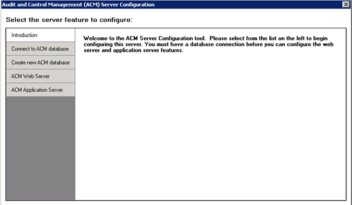
Once the Utility opens you will see this screen:
Let’s start by creating a new ACM database. Click ‘Create new ACM database’, enter the database server\instance name and the name of the database to create. Finally, click ‘Create’ and wait.
When done, click ‘Connect to ACM database’ to verify that the connection info for the database has been successfully stored there. If required set up the connection here and hit ‘Save’.
Now that we have configured the database and the connection to the database, we need to setup the ACM Web Server and ACM Application Server.
Click ‘ACM Web Server’ to get started and choose where you will create the Web Site. Since I had an empty IIS install, I chose Default Web Site. I entered a new for the web application and made sure to use correct credentials for the Application Pool Identity. Also, specify an initial Central Administrator account and click ‘Create’.
Then we can continue to the ACM Application Server configuration; click ‘ACM Application Server’ to get started. Here we will need to specify the URL of the Web Server you have just configured (in my case it was just http://localhost/ACM). Optionally you can specify users whose file saves you would like to ignore. When done do not forget to click ‘Save’. Now you can click on ‘Show Service Manager’ to jump to the other tool we will need (Microsoft Office ACM Service Manager).
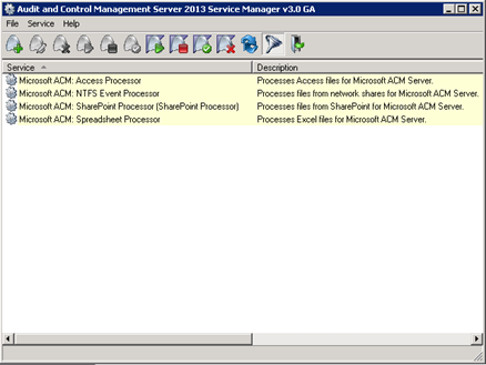
When the ACM Service Manager opens it should show you four services (see screenshot below).
You will need to configure the services correctly. In my experience it works best if you first stop the service (right-click, Stop) before editing them (right-click, Edit). You will need to specify a logon account and password for each service on the Settings tap of the properties dialog box. Also I chose to change the start-up mode for each service to Automatic. Once done your services should all be started (you can check the status in the service manager). If not you may have to start them by hand.
Note that you do not have to run all services. For example if you do not want to monitor SharePoint libraries, you do not have to configure this service. Also, if you do not want to monitor Access files, you do not have to configure the Access Processor service. The NTFS Event Processor service is required is you want to monitor file shares. The Spreadsheet Processor service is require for monitoring Excel files.
Now open up your browser and navigate to your ACM Web Server (in my case http://localhost/ACM).
You will see a page titled ‘My Files’ and it will be empty. Don’t worry, we will fix that very soon.
Click on the little gear icon right next to your name in the top right and click ‘Site Settings’ to open the settings. You can always go here if you need to troubleshoot. Service Status and Event Log are two very helpful items to check out first if you are having problems.
For now, click on Processing Folder. Here, specify a UNC path where the Excel and Access processor can store files while processing. This folder will be emptied regularly, so don’t worry too much about this. Anyway, I choose to create a file share on my local server for this purpose and entered the share name here. When done, click ‘OK’.
Next up is the File Processor Aliases option. Here you can specify the aliases of processors to use to scan items. The default alias (AppSrvAlias) should already be added. If not, add it and return to the previous screen.
The last item we need to look at is Monitored Folders. Here you can set up the folders to monitor. I used a file share to monitor for files since I do not have SharePoint installed on this machine. You can add multiple folders to monitor and mix both types. When specifying a file share folder you will of course need to enter the UNC path and you could change the file types to monitor (although I recommend leaving it like it is). Also you can specify if you also want to monitor subfolders. The Change Tracking option specifies the tracking level for Excel files, which determines how deeply you want to investigate Excel files. I chose ‘Functional, Formatting and Data Entry’ but ‘Functional’ is recommended, since you will probably not be interested in formatting changes like colors and fonts. However, I found Data Entry to be interesting to track, so that is why I chose that level of tracking.
You can specify if you want to track changes each time the file is saved or once a day at a certain moment.
An important setting is the processing folder, which is used to store versions of monitored files. Enter a UNC path in here which is different from the processing folder and the monitored folders specified earlier. Also bear in mind that users should not be given access to this folder. The number of versions to store per file is configurable here also.
Finally, we need to specify folder manager and viewer permissions and click ‘OK’.
Repeat this process for every folder you want to monitor and you’re done configuring ACM.
If you now create a new file or edit any existing file in one of the monitored locations you should see it showing up on the My Files page. In the case of Excel files you will need to make a change that actually triggers the tracking level you specified. If you went with the ‘Functional’ setting and make a formatting change it will not be tracked.
In my next blog I will show what you can do with monitored files, so stay tuned!
 Dutch Data Dude
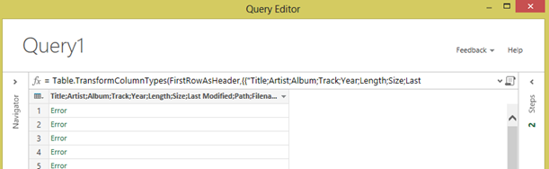


 icon to select the columns to expand from your Excel sheet and click ‘OK’.
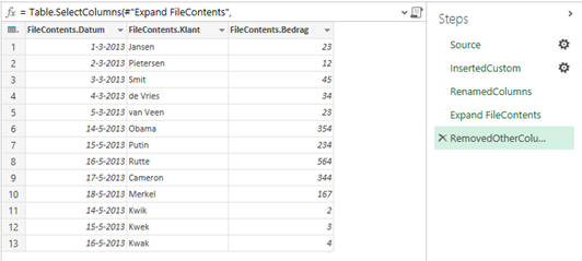
 . Click it and the contents of the files is combined together and shown in a new column (Column1):
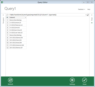
 ) and choose ‘Use First Row As Headers’.